RAG ChatBot
 Mahesh Kumar
Chapter 1: Why RAG Exists
Every leap in technology begins with a limitation. For language models, that limitation was memory.
They could write poetry, fix bugs, and summarize history — but ask them about a breaking event or a company's internal rulebook, and they'd stall. Not because they lacked intelligence, but because they lived in a frozen snapshot of time.
That's where Retrieval-Augmented Generation, or RAG, entered the picture — quietly but powerfully.
RAG isn't just a clever add-on; it's the missing half of modern intelligence systems. It bridges the gap between what the model knows and what the world knows now.
The Locked Library
Think of a large language model like a brilliant scholar locked inside a vast library that closed five years ago. It remembers every page but hasn't read a single new book since.
Now, if you ask about "Top AI startups in 2026", this scholar can only guess based on 2021 or 2022 data.
RAG hands that scholar a new ability — to walk out, fetch the latest data, and respond with current, evidence-backed information.
That's what makes RAG special: it lets AI act like a researcher, not a storyteller.
The Core Idea
At its heart, RAG works like this:
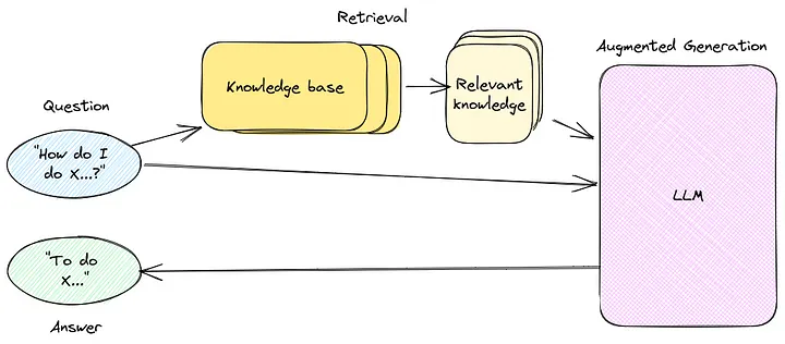 RAG Pipeline Overview
- User asks a question → "What's our company's remote work policy?"
- System retrieves relevant documents → Fetches HR policy PDFs, recent emails
- Model reads context → Understands the specific rules
- Generates grounded answer → Responds with accurate, current information
It's deceptively simple, but each step hides a small marvel of engineering.
A Hands-On Example
Let's say someone wants to know:
"What's the refund policy for our software product?"
A normal model might respond:
"Refunds are typically available within 30 days."
That's generic — maybe even wrong.
But a RAG-enabled system can read your company's actual policy PDF and give a factual answer:
"Refunds can be requested within 14 days of purchase, provided the license hasn't been activated."
Here's a mini RAG prototype built using Python and LangChain:
from langchain.document_loaders import PyPDFLoader
from langchain.text_splitter import RecursiveCharacterTextSplitter
from langchain.embeddings.openai import OpenAIEmbeddings
from langchain.vectorstores import FAISS
from langchain.chains import RetrievalQA
from langchain.llms import OpenAI

# Load the refund policy document
loader = PyPDFLoader("RefundPolicy.pdf")
documents = loader.load()

# Split into manageable chunks
splitter = RecursiveCharacterTextSplitter(chunk_size=500, chunk_overlap=50)
chunks = splitter.split_documents(documents)

# Create vector embeddings
embeddings = OpenAIEmbeddings()
db = FAISS.from_documents(chunks, embeddings)

# Build the QA chain
qa = RetrievalQA.from_chain_type(
    llm=OpenAI(model="gpt-4-turbo"),
    retriever=db.as_retriever(),
    return_source_documents=True
)

# Ask a question
query = "What is the refund policy for the software?"
response = qa({"query": query})
print(response["result"])
What happens here?
- The PDF is broken into small sections, each turned into a vector — a kind of numeric fingerprint
- When the user asks a question, the system retrieves only those fragments that are semantically closest to the query
- The LLM then reads that data, understands context, and answers precisely
That's the basic magic of RAG — retrieval grounds generation.
The Turning Point
Before RAG, there were two main ways to improve model accuracy:
- Fine-tuning: Retrain the model with new examples (expensive and slow)
- Prompting: Feed the model new info every time you ask something (manual and inefficient)
RAG introduced a third way: fetching the right context dynamically.
- No retraining
- No manual prompt stuffing
- Just smart retrieval and generation
Why It Feels So Human
What's fascinating is that this mechanism mirrors how people think.
Humans don't store every fact. They remember where to find it.
When asked, "What's the population of Tokyo?", no one memorizes the number — they know how to look it up. RAG gives AI the same gift: not memory, but access.
This subtle difference changes everything. It means an AI system doesn't have to know everything — it just needs to know where to look and how to reason.
Small Experiment You Can Try
To see RAG's difference in action, try this simple test:
-
Ask a normal model (without retrieval): "When did OpenAI release GPT-4?"
-
Now feed it context:
Context: GPT-4 was released on March 14, 2023. Question: When was GPT-4 released? -
Compare responses.
The second answer will be direct and certain, because it's context-anchored. That's what RAG automates — it builds that context dynamically, every time.
Chapter 2: Naive and Neural Retrieval
Every retrieval system — from search engines to AI assistants — walks the same line: finding what's relevant.
The trick lies in how relevance is defined.
For some systems, relevance is just matching words. For others, it's matching meaning. That distinction, simple as it sounds, defines the gulf between naive retrieval and neural retrieval — the old world and the new.
The Naive Retriever
Imagine asking a librarian, "Show me everything about solar panels." She returns every book that contains the word "solar" — novels, cookbooks, even a poetry collection called Under the Solar Sky.
That's naive retrieval in a nutshell.
It doesn't understand the question. It just matches strings.
In machine terms, naive retrieval uses tools like:
- TF-IDF (Term Frequency–Inverse Document Frequency)
- BM25 (used by search engines like Elasticsearch)
- or even simple SQL
LIKE '%word%'queries
They work by counting how often words appear, ranking documents by overlap frequency. It's fast, cheap, and utterly blind to meaning.
 Keyword vs Semantic Search
Let's see this in action.
Naive Keyword Retrieval
from sklearn.feature_extraction.text import TfidfVectorizer
from sklearn.metrics.pairwise import cosine_similarity

# Sample documents
docs = [
    "Solar panels convert sunlight into electricity.",
    "The moonlight glows at night.",
    "Wind turbines generate renewable power."
]

# Create TF-IDF vectors
vectorizer = TfidfVectorizer()
tfidf_matrix = vectorizer.fit_transform(docs)

# User query
query = ["energy from sunlight"]
query_vec = vectorizer.transform(query)

# Compute similarity
scores = cosine_similarity(query_vec, tfidf_matrix).flatten()

# Rank results
for idx in scores.argsort()[::-1]:
    print(docs[idx], "→", round(scores[idx], 2))
Output:
Solar panels convert sunlight into electricity. → 0.52
Wind turbines generate renewable power. → 0.08
The moonlight glows at night. → 0.00
Looks reasonable, right? It found "sunlight."
But here's the problem — change the query slightly:
query = ["renewable energy from the sun"]
Output:
Wind turbines generate renewable power. → 0.19
Solar panels convert sunlight into electricity. → 0.00
Now it fails completely because it doesn't recognize that "energy from the sun" means "solar energy." No overlap in words, no match — even though semantically, it's a perfect fit.
That's the naive retriever's curse — literal loyalty, semantic blindness.
The Neural Retriever
Neural retrieval, on the other hand, doesn't care about words — it cares about meaning.
It transforms text into embeddings — numerical vectors that represent the concept of a sentence. Two sentences with similar meanings will have embeddings that lie close together in a high-dimensional space.
Think of it as clustering thoughts, not words.
The simplest way to feel this difference is to visualize it. Imagine plotting the words "sun," "solar energy," "light," "wind turbine," "moon" in a 3D space. You'd see sun and solar energy floating near each other, while moon drifts away.
That's semantic proximity.
Neural Retrieval Using Sentence Embeddings
Let's rebuild the same example with semantic search.
from sentence_transformers import SentenceTransformer, util

# Model for embeddings
model = SentenceTransformer('all-MiniLM-L6-v2')

# Same documents
docs = [
    "Solar panels convert sunlight into electricity.",
    "The moonlight glows at night.",
    "Wind turbines generate renewable power."
]

# Encode documents and query
doc_embeds = model.encode(docs, convert_to_tensor=True)
query = "renewable energy from the sun"
query_embed = model.encode(query, convert_to_tensor=True)

# Compute cosine similarities
scores = util.cos_sim(query_embed, doc_embeds)[0]

# Rank results
for idx in scores.argsort(descending=True):
    print(docs[idx], "→", round(scores[idx].item(), 3))
Output:
Solar panels convert sunlight into electricity. → 0.87
Wind turbines generate renewable power. → 0.55
The moonlight glows at night. → 0.21
That's it — same idea, new intelligence. No matching words, yet perfect understanding. The model knows that "energy from the sun" relates to "solar panels."
This difference might look small in a toy example, but in a real RAG system handling millions of documents, it's monumental.
Why It Matters for RAG
RAG relies entirely on retrieval quality. If the retriever fails, the LLM hallucinates or answers vaguely.
That's why modern pipelines almost always use vector databases and semantic embeddings for retrieval.
Yet, this doesn't mean naive retrieval is obsolete. In fact, many enterprise RAG systems use a hybrid approach:
- Keyword search (BM25) for precision
- Vector search for conceptual recall
The retriever then blends both scores to find the best candidates.
Hybrid Retrieval Logic
def hybrid_score(bm25_score, vector_score, alpha=0.6):
    return alpha * vector_score + (1 - alpha) * bm25_score
In practice, systems like Weaviate, Elasticsearch with dense vectors, or Pinecone hybrid search handle this fusion internally. You get the speed of keyword lookup and the depth of semantic understanding — the best of both worlds.
Why Naive Retrieval Still Exists
Let's be fair — naive methods have their charm. They're lightning fast, resource-light, and predictable. For FAQs or small datasets where vocabulary overlaps are high, TF-IDF or BM25 works beautifully.
But once you deal with real-world text — human writing with nuance, abbreviations, typos, and synonyms — naive methods start falling apart.
That's where neural retrieval feels almost human.
Chapter 3: Vector Databases Explained
Every great memory system — human or machine — needs structure.
Humans store memories in patterns, linked by association and context. Machines, surprisingly, do something very similar. In the world of AI, that structure lives inside something called a vector database — the quiet engine of retrieval-augmented generation.
From Words to Numbers
Before understanding what a vector database does, it helps to understand what it stores.
A model doesn't think in words. It thinks in numbers. Each word, sentence, or paragraph gets transformed into a long list of floating-point values — hundreds or thousands of them — called a vector.
A single vector might look like this:
[0.13, 0.72, -0.48, 0.66, ... , 0.19]
Each number represents a feature the model has learned to recognize — things like tone, subject, or semantic meaning. When two pieces of text have similar meanings, their vectors end up close to each other in this vast mathematical space.
Now imagine millions of those vectors, each representing a sentence from books, PDFs, or research papers. Finding the most relevant ones to a query becomes a search problem.
And that's where the vector database comes in.
Why Normal Databases Don't Work
Traditional databases — SQL or NoSQL — are built to handle exact matches: numbers, names, IDs. They're brilliant for structured data but terrible at meaning-based search.
You can't just ask PostgreSQL, "Show me text that feels similar to 'benefits of green energy'." It doesn't understand "feels similar."
Vector databases, on the other hand, are built for approximate nearest neighbor search — often abbreviated as ANN. Instead of matching exact values, they find vectors closest in meaning.
These databases rely on specialized indexing algorithms like:
- HNSW (Hierarchical Navigable Small Worlds)
- IVF Flat (Inverted File Index)
- PQ (Product Quantization)
These terms sound complex, but they all exist for one reason: to make similarity search blazingly fast, even when storing millions of entries.
Building a Mini Vector Database
Let's try a small experiment using FAISS, an open-source library developed by Facebook AI.
from sentence_transformers import SentenceTransformer
import faiss
import numpy as np

# Step 1: Create some sentences
sentences = [
    "Solar energy is renewable and clean.",
    "Wind turbines generate electricity.",
    "The moon reflects sunlight at night.",
    "Nuclear power plants use uranium.",
]

# Step 2: Convert them into embeddings
model = SentenceTransformer('all-MiniLM-L6-v2')
embeddings = model.encode(sentences)

# Step 3: Create a FAISS index
dimension = embeddings.shape[1]
index = faiss.IndexFlatL2(dimension)

# Step 4: Add embeddings to the index
index.add(np.array(embeddings))

# Step 5: Search for a query
query = model.encode(["clean renewable energy"])
distances, indices = index.search(np.array(query), k=2)

# Step 6: Display results
for i, idx in enumerate(indices[0]):
    print(sentences[idx], "→ distance:", round(distances[0][i], 3))
Output:
Solar energy is renewable and clean. → distance: 0.18
Wind turbines generate electricity. → distance: 0.42
That's the magic right there — no keyword overlap, no training, yet perfect retrieval.
The vector database doesn't read text; it reads meaning.
How It Fits in the RAG Pipeline
The role of a vector database in RAG is simple but critical:
- Store document embeddings along with metadata (like document title or source)
- Retrieve the most semantically similar chunks when a query comes in
- Feed those chunks into the model's prompt for context-based generation
That retrieval stage — the quiet moment before the model speaks — depends entirely on the quality of the vector index.
Using ChromaDB
Here's how ChromaDB works as a local, simple-to-use vector store.
from langchain.vectorstores import Chroma
from langchain.embeddings import OpenAIEmbeddings
from langchain.text_splitter import RecursiveCharacterTextSplitter
from langchain.document_loaders import TextLoader

# Step 1: Load and split text
loader = TextLoader("tech_articles.txt")
docs = loader.load()
splitter = RecursiveCharacterTextSplitter(chunk_size=500, chunk_overlap=50)
chunks = splitter.split_documents(docs)

# Step 2: Create embeddings
embeddings = OpenAIEmbeddings()

# Step 3: Initialize Chroma store
vectorstore = Chroma.from_documents(
    chunks,
    embeddings,
    persist_directory="chroma_index"
)

# Step 4: Query
query = "What are the latest trends in machine learning?"
results = vectorstore.similarity_search(query, k=3)

for res in results:
    print(res.page_content[:200], "...")
The output returns text chunks that mention ML trends, frameworks, or research — all without storing any explicit keywords. The Chroma store remembers context semantically, letting RAG feed meaningful content into the LLM.
Combining Keywords and Meaning
Sometimes, semantic retrieval alone isn't enough. If you search "tech startups in Bangalore," you want results from Bangalore, not startups generally.
Vector similarity doesn't enforce location or metadata filters by default — that's where hybrid search comes in.
Many modern databases (like Weaviate and Pinecone) support metadata filtering, which combines keyword-based constraints with vector search.
For example:
results = vectorstore.similarity_search_with_score(
    "tech startups in Bangalore",
    k=5,
    filter={"city": "Bangalore"}
)
This ensures the context matches both the meaning and the specific filter criteria.
Hybrid search merges the precision of old-school retrieval with the understanding of neural embeddings.
Scaling Beyond Local Storage
FAISS and Chroma work beautifully for small datasets — say, a few thousand documents. But when the index grows to millions of chunks, performance drops.
That's where Pinecone or Weaviate Cloud steps in.
They're built for production-level RAG — distributed storage, vector compression, caching, and automatic scaling.
For instance, in Pinecone, adding and querying vectors looks like this:
import pinecone

pinecone.init(api_key="your_key", environment="us-east1-gcp")
index = pinecone.Index("rag-index")

# Upsert vectors
index.upsert([
    ("doc1", embedding_vector, {"title": "Refund Policy"}),
    ("doc2", another_vector, {"title": "Admission Rules"})
])

# Query
query_vector = model.encode("how can I apply for a refund?")
result = index.query(
    vector=query_vector.tolist(),
    top_k=3,
    include_metadata=True
)
Within milliseconds, Pinecone retrieves the most semantically relevant chunks, even from millions of entries.
Why This Matters for Real-World AI
Vector databases are what make systems like Perplexity AI, ChatGPT with browsing, and Notion AI capable of grounding their responses.
They're the memory vaults of context — efficient, meaning-aware, and lightning-fast.
Without them, every query would be a blind guess or an expensive full-text search.
By indexing knowledge once and retrieving smartly, RAG systems become both cost-effective and intelligent — able to answer deeply while staying grounded.
Mini Project Challenge
Here's a small experiment worth trying:
- Collect 20 short articles about AI, startups, or technology trends
- Load them into Chroma or FAISS as chunks
- Ask queries like:
- "Which companies are working on autonomous vehicles?"
- "What are the latest developments in quantum computing?"
- Observe how vector retrieval finds correct passages, even when the query wording changes
This small project will show firsthand how retrieval makes AI feel intelligent.
Chapter 4: The RAG Pipeline
Every intelligent system needs a process — a rhythm that connects raw data to thoughtful output. For RAG, that rhythm is the pipeline.
It's not a single function or an API; it's a carefully tuned orchestra of tasks that move knowledge from storage to speech.
Think of it like this: RAG is the concept, the philosophy. The RAG pipeline is its anatomy — the bloodstream through which context, meaning, and language flow.
In this chapter, that anatomy will be unfolded layer by layer, with working examples and a few insights that make the abstract mechanical heartbeat of retrieval-augmented generation easier to grasp.
The Essence of a Pipeline
A RAG pipeline is the chain of stages that transforms static data into a dynamic, knowledge-grounded answer.
It always moves in this order:
 RAG Pipeline Flow
User Query → Retrieval → Augmentation → Generation → Response
Each stage hands off something valuable to the next — like a relay team where every runner knows their job.
The pipeline exists for one reason: to make knowledge usable.
A model like GPT-4 can write, reason, and infer, but it doesn't know your documents or the latest web updates. The pipeline's job is to bring that missing information into its reach.
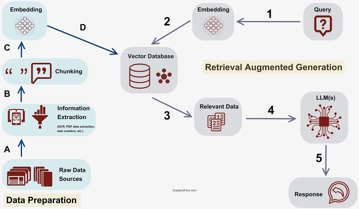
Step 1: Indexing
Indexing is where everything begins. You feed the system your data — reports, PDFs, research notes, academic journals, policies — and it transforms them into machine-searchable meaning.
Imagine throwing a hundred books into a blender and somehow being able to retrieve the exact sentence you need later. That's what indexing does.
Here's what indexing typically involves:
- Document Loading — Collecting the source data
- Chunking — Breaking large texts into manageable pieces
- Embedding — Turning each chunk into a numerical vector
- Storing — Saving those embeddings in a vector database
Let's see it in practice:
from langchain.document_loaders import PyPDFLoader
from langchain.text_splitter import RecursiveCharacterTextSplitter
from langchain.embeddings import OpenAIEmbeddings
from langchain.vectorstores import FAISS

# Step 1: Load the document
loader = PyPDFLoader("Tech_Guidebook.pdf")
docs = loader.load()

# Step 2: Split text into smaller chunks
splitter = RecursiveCharacterTextSplitter(
    chunk_size=800,
    chunk_overlap=100
)
chunks = splitter.split_documents(docs)

# Step 3: Create embeddings
embeddings = OpenAIEmbeddings()

# Step 4: Build a FAISS vector index
db = FAISS.from_documents(chunks, embeddings)
That's indexing in its simplest form — taking unstructured text and turning it into a searchable knowledge base.
Why chunk the data? Because models can't process a hundred pages at once, and smaller chunks help the retriever find just the right piece of context later.
Step 2: Retrieval
Once data is indexed, retrieval is how RAG "remembers."
When a user asks a question, the system embeds that query into the same vector space as the stored documents and finds the closest matches.
It's almost poetic: the query and the document vectors meet in a multidimensional space — and proximity means relevance.
Here's a hands-on version:
query = "What are the best practices for building scalable APIs?"
query_embedding = embeddings.embed_query(query)
retrieved_docs = db.similarity_search_by_vector(query_embedding, k=3)
Under the hood, FAISS calculates which chunks of text lie closest to the question vector using cosine similarity.
The k=3 parameter ensures it retrieves the top three relevant passages.
The retriever, at this point, isn't answering the question — it's just finding the context to help the LLM answer later.
Step 3: Augmentation
Now comes the elegant part — augmentation. This is where retrieval meets reasoning.
The retrieved chunks are injected into the model's input prompt, giving it a factual base to think from. Instead of relying on its own training memories, the model now reads directly from your documents.
Here's a simplified look:
context = "\n\n".join([doc.page_content for doc in retrieved_docs])

prompt = f"""
You are a helpful assistant. Use the context below to answer the user's question accurately.

Context:
{context}

Question:
{query}
"""
This augmented prompt is then sent to the LLM:
from langchain.llms import OpenAI

llm = OpenAI(model="gpt-4-turbo")
response = llm(prompt)
print(response)
Suddenly, the model's answers become grounded — not just articulate, but reliable.
Ask it, "What's the recommended architecture for microservices?" It won't hallucinate anymore. It'll tell you what's actually written in the guidebook you indexed.
Step 4: Generation
The LLM is now speaking, but not from thin air. It's reasoning with evidence.
This stage is called generation, but what makes it remarkable is its constraint.
Traditional generation is free-flowing — creative but unreliable. RAG-based generation is focused — factual, document-aware, and transparent.
If you enable return_source_documents=True, you even get references along with the answer:
from langchain.chains import RetrievalQA

qa_chain = RetrievalQA.from_chain_type(
    llm=OpenAI(model="gpt-4-turbo"),
    retriever=db.as_retriever(),
    return_source_documents=True
)

result = qa_chain({
    "query": "Which framework is best for real-time applications?"
})

print(result["result"])
print("\nSources:", result["source_documents"])
Now your chatbot isn't just saying something; it's citing where it came from — exactly like a researcher does.
Step 5: Response
Finally, the user sees the answer — clean, human-like, and backed by context.
This last step might seem trivial, but it's where all the hidden machinery pays off. A smooth UI, a clear tone, and even a confidence score can make the experience feel magical.
In production, this layer is often integrated with frameworks like Streamlit, Gradio, or React — building conversational dashboards powered by RAG under the hood.
Putting It All Together
Here's a minimal end-to-end pipeline code block for reference:
from langchain.chains import RetrievalQA
from langchain.document_loaders import PyPDFLoader
from langchain.embeddings import OpenAIEmbeddings
from langchain.text_splitter import RecursiveCharacterTextSplitter
from langchain.vectorstores import FAISS
from langchain.llms import OpenAI

# Indexing
docs = PyPDFLoader("Tech_Guidebook.pdf").load()
chunks = RecursiveCharacterTextSplitter(
    chunk_size=800,
    chunk_overlap=100
).split_documents(docs)
embeddings = OpenAIEmbeddings()
db = FAISS.from_documents(chunks, embeddings)

# Retrieval + Generation
retriever = db.as_retriever(search_kwargs={"k": 4})
qa_chain = RetrievalQA.from_chain_type(
    llm=OpenAI(model="gpt-4-turbo"),
    retriever=retriever
)

# Query
query = "List the best practices for API security"
answer = qa_chain.run(query)
print(answer)
This small script captures the entire journey — from text to context to cognition.
Modular Thinking
The beauty of the RAG pipeline is its modularity. Each part can evolve independently:
- Swap FAISS for Pinecone or Chroma for scalability
- Replace OpenAI embeddings with SentenceTransformers or Cohere for cost optimization
- Add re-ranking layers like Cohere's Rerank API for sharper context selection
- Introduce context compression models to summarize retrieved data when context windows are limited
This flexibility is what makes RAG pipelines so adaptable — you can scale them from a local notebook to an enterprise AI platform with minimal friction.
The Detective Analogy
Picture a detective (the LLM) and an assistant (the retriever).
The assistant runs to the archives, digs through records, and brings back the most relevant case files. The detective reads them, connects the dots, and presents a conclusion — backed by evidence.
That's exactly how the RAG pipeline works — one retrieves, one reasons. And together, they create something neither could do alone: intelligent, grounded, trustworthy answers.
Final Thoughts
RAG isn't just a technical pattern — it's a philosophical shift in how we think about AI.
Instead of building systems that pretend to know everything, we're building systems that know how to find out.
That's closer to how humans actually work. We don't memorize the world; we navigate it.
RAG gives machines that same gift — the ability to reach beyond their training, to look up, to verify, to cite.
And in doing so, it transforms AI from a storyteller into a scholar.